Using a Monte Carlo Program to Define Process Control Parameters
© Ken Osborn 2013
Abstract: Profiler is a program written in Excel® Visual Basic® and uses a Monte-Carlo simulation to fit process data to a Normal distribution. Output includes raw data and simulation statistics and outliers are identified and flagged. If the data are not skewed and show a good fit except for the outliers, process control limits can be calculated from the Normal curve average and standard deviation.
The Problem
Controlling any production process like weight of material added to a mix, treatment and discharge of a waste product, or analysis of a material requires that the variance be predictable. When a process exceeds the established variance it is out-of-control. Process control parameters include the process average, standard deviation, and control limits. Control limits are frequently set at the average plus or minus three standard deviations.
The difficulty with this approach is that if the statistics used to set the control limits are generated when the process is out-of-control they will overestimate the acceptable range of variance by including outliers that may not be initially suspect. This may be particularly true at process startup when there is no baseline of data.
The Solution
To avoid the problems of outliers driving the process control statistics, the control limit statistics can be derived from a Normal distribution fitted to the process data. The Normal distribution will exclude outliers and more closely reflect the variance in the process output when it is under control.
Profiler, a program written in Excel, fits a Normal curve to a data set using a Monte Carlo simulation. The fit is iterative starting with an initial guess which checks for fit against the 25th and 75th percentiles of the data. Adjustments are made to the mean and standard deviation of the simulation until a pre-set error is achieved based on the 75th percentile. The error is optimized for low error vs time for convergence. Output consists of 100 data points, simulation mean, standard deviation, 25th, 75th, and 99th percentiles, and flags all values in the original data set exceeding one standard deviation of the 99th percentile.
An Example
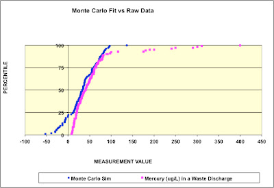
Data plotted in red in Chart 1 are from a waste discharge stream controlling for mercury. Clearly some of the values are outliers and do not represent the process when it is in control.

Chart 1: Mercury in discharge vs Monte Carlo simulation
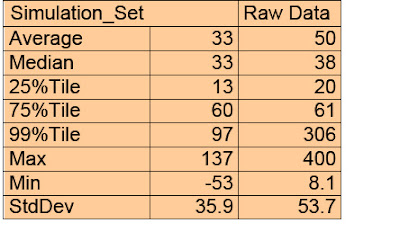
The blue line represents the Monte Carlo fit to a Normal distribution. The majority of the mercury discharge data exhibit a close fit to the simulation curve with outliers clearly visible. The statistics for the mercury and simulation results (Table 1) show the divergence from normalcy at the extreme ends of the distribution. Of course, we are only concerned about the high outliers that would drive the statistics if retained. Using the raw data, a 3-sigma upper control limit (3S UCL) calculates as 240 while the simulation UCL is 141.
Since the raw data clearly include results from the process when it was out of control, outliers should be excluded. But which ones? Using the raw data 3S UCL leaves several high values that could misrepresent the process when in control. Conversely, using the simulation UCL may remove more values than justified. Using an alternative determination of 1 standard deviation above the 99%tile (UCL_PTile), the simulation UCL_PTile is 133. If the raw data 3S UCL is used, there are six outliers (240, 250, 290, 300,310, and 400). If the simulation UCL_PTile value is used, there are ten outliers (175, 180, 190, 200, 240, 250, 290, 300, 310, 400). These are the values plotted in red at the extreme right in Chart 1.

Table 1: Comparison of Monte Carlo and Raw Data Statistics
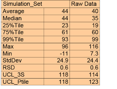
When the 3S UCL is recalculated for the raw data excluding the outliers exceeding the simulation UCL_Ptile, the statistics for the raw data are comparable to the simulation (Table 2). In addition, whether the 3S UCL or the UCL_PTile is used makes little difference. Once the outliers have been identified, the data represent a process that is predictable.

Table 2: Process statistics after removal of outliers
Conclusion
Statistical control of a process requires establishing realistic control limits based on data that represent the process in control. At startup the process may not be in control and include outliers. Fitting the data to a Normal curve from which the control statistics are derived provides a simple mechanism to identify the outliers and establish statistical process control limits. A Monte Carlo simulation can be used to fit the data to a Normal curve.
If you would like a copy of the 'Profiler' program, please write me. You may use the program for your own purposes or post on your blog with credit. You may not use the program for commercial purposes. Write me at kozborn@sbcglobal.net.


