The Outlier Paradox and Global Warming

The Outlier Paradox and Global Warming

© Ken Osborn

Feb 2012

Hot winters ahead?  I can’t say for sure, but this last January seemed a lot warmer than a couple years ago when the winter was mild.  I checked the records for the city of Oakland (airport) and the daily highs for Jan 2012 averaged 2.3 degrees Fahrenheit (dF) warmer than Jan 2010.  That doesn’t seem like a lot.  But when I checked for the warmest days in 2010 and compared them to 2012 I saw that my impression that it seemed warmer this year than in 2010 was correct.  In 2010 two of the Jan daily high temperatures exceeded 60 dF and in 2012 there were 7 days in Jan exceeding 60 dF. 

So my impression that this winter was warmer was based not on the average of the daily high temperatures but rather the number of warmer than typical days.  This I call the Outlier Paradox: increasing means accelerates extremes.  Small changes in a data set's average are associated with large changes in the frequency of values exceeding some threshold value: these extreme values are also referred to as outliers.  This is a statistical property of numerical distributions, as I will try to explain.

Measurements repeatedly performed on any item and collected into a data set are frequently randomly distributed.  Given a large enough data set, if the individual results are randomly distributed, the shape of the plotted numbers will be symmetrical: values exceeding the average will balance nicely against numbers below the average in a mirror image fashion.  This is called a Normal distribution.  So are temperature records Normally distributed? 

Chart 1 is a plot of the Jan 2012 daily high temperature readings for the City of Oakland.  The data are ranked from low to high and plotted against the probability that a given measurement will exceed all other measurements in the set.  Except for the four highest values, the plotted temperature readings (red) nicely fit the curve for a Normal distribution (blue).  The curve is symmetrical around the center with roughly the same number of readings on either side.  Measurements close to the center have a higher probability and measurements far from the center a lower probability.  This is visualized by the flattening of the curve at the extreme ends. 

Chart 1: Testing temperature readings for Normality

An interesting property of Normal distributions is that even large changes in the extreme values have a smaller effect on the average.  When examining changes over time, averages only may be a poor predictor of environmental impacts if the outliers are ignored.  

As an example, see Chart 2.  Data set 1 represents a collection of measurements with an average of 100 and a standard deviation of 10%.  Approximately 4 out of 1000 measurements will exceed a threshold of 125.  Change the average to 105 and the number of measurements exceeding 125 increases to 16 out of 1000.  A 5% change in the average becomes a 400% change in the values exceeding a threshold just 25% above the average (100*16/4 = 400%).  An increase in the standard deviation will magnify the spread of extreme values even more. 

Chart 2: A small change in the mean is associated with large changes in the frequency of outliers

This property holds for any set of measurements taken over time when the distribution is Normal.  Records of rainfall, temperature, atmospheric pressure, and number of cars per hour passing a given point on the freeway can all be treated as Normal distributions.  Even though there are causal factors associated with each of these, any given measurement is randomly determined relative to the measurements that immediately precede or follow.  Though we know it may rain tomorrow, the exact number of inches of rain that will fall is an unknown until after the event.  

Returning to the records for the City of Oakland for Jan of 2010 and 2012, let’s take a statistical look at the distribution of daily high readings (Chart 3).  The average high temperature for Jan 2010 was 55.7 degrees Fahrenheit (dF) and the variance as measured by the standard deviation was 2.6 dF.  For 2012 the Jan average high temperature was 58 dF and the standard deviation 4.9.  Using the lower 2010 variance for both years, the fitted Normal curves predict 5% of days exceeding 62 dF for 2012 and 0.8% for 2010.

Chart 3: Comparison of Jan High Temperatures for 2010 and 2012 using 2010 Variance

Chart 3 demonstrates the effect of changing the mean of a distribution of data but not the standard deviation.  The curve shifts horizontally to the right for an increase in the mean with each individual point moving the same amount so that the two curves are parallel to each other. 

Of course the variance was not the same for the two years, and when the change in variance is considered (Chart 4), the differences are even greater with a prediction of 21.8% of the days exceeding 62 dF for 2012 compared to the 0.8% for 2010. 

Chart 4: Comparison of Jan High Temperatures for 2010 and 2012

When both the standard deviation and mean are changed, the curve not only shifts laterally but also rotates.  Chart 5 using a hypothetical set of temperature demonstrates what happens when the mean is fixed mean but the standard deviation changes.  Here the curve rotates around the center but the center does not move horizontally.   Thus if two sets of temperature records (or any measurement records) have the same average but different standard deviations, the set with the higher standard deviation will have more extreme values at both the high and low temperatures.   

Chart 5:  Changing only the standard deviation rotates the curve around the mid-point

  

The extra warm days of Jan 2012 should not be taken in isolation to determine whether global warming is a reality.  These data represent a narrow temporal and spatial snapshot.  Next winter may bring even warmer winter days or it could bring winter lows that are the lowest of the decade.  While we might take note of unusually extreme temperatures, it is the preponderance of data that must answer the question of whether an apparent trend is merely a statistical excursion or a real trend.  

Ref: http://www.wunderground.com/history/airport/KOAK/2010/1/1/MonthlyHistory.html?req_city=NA&req_state=NA&req_statename=NA

Predator - Prey: Part III - The Interactive Model

Forage (aka carrying capacity) feeds the deer; deer feed the wolves; wolves keep the deer herd in balance with the forage.  It's a nice model, but things don't always work that smoothly.  Two previous posts discuss a mathematical model written in Excel that interactively explores some of the possible outcomes given initial conditions of deer herd size, number of wolves, intrinsic growth rates of deer and wolves, and the carrying capacity and carrying capacity variance factor.  This latter is a random card designed to incorporate the unpredictable effects of climatic variation, forage decline, or other things that can change the amount of forage but are not predictable from one year to the next.

Previous posts on this topic are at:


http://misterkenblog.blogspot.com/2012/01/predator-vs-prey-mathematical-model.html
http://misterkenblog.blogspot.com/2011/12/predator-vs-prey-will-wolves-dominate.html

Ready to try you hand at creating your own scenarios?  A simplified interactive model programmed in an Excel spreadsheet is available for the curious in Google Docs at
https://docs.google.com/spreadsheet/ccc?key=0AixHzIqC4EIYdGJ6VFgyLUl3UERKUEF4RUw1Z0dVMkE

There are eight variables in the model you can work with shown in the diagram below.

The population size of the deer herd (here it is 5000), deer growth rate, carrying capacity for the deer herd, variance in carrying capacity (K), wolf population (here it is 10), wolf pack growth rate, predator efficiency, and number of deer required for wolf survival.  You can change any and all of these starting numbers to see what happens.  For example, to evaluate the effect of dramatic swings in climate try changing the variance in K (now at 2000) to a higher or lower number.  A higher number would represent greater unpredictability and a lower number a more stable environment.

Have fun.

Predator vs Prey - A Mathematical Model - Part 2 of a 3 Part Series

In the first installment of my predator-prey model I presented graphs of population growth under three scenarios that included deer and forage but no predators.  Scenario 1 was for a stable environment (i.e, constant carrying capacity): the deer herd rapidly grew from a starting population until it reached the carrying capacity then leveled out.  Scenario 2 was a moderately variable environment and the deer initially grew but the population fluctuated above and below the carrying capacity.  Scenario 3 was for a highly variable environment.  In this last case, the deer herd grew, fluctuated in number, then crashed and died out.  For a more complete review see http://misterkenblog.blogspot.com/2011/12/predator-vs-prey-will-wolves-dominate.html.

What happens when predators are introduced?  Will the deer herd die out sooner or will it stabilize because wolves keep the deer herd in check with the environment?  Can predictions even be made?  Let's see.

Scenario 1: Start with a deer herd well below the carrying capacity, a small number of wolves, and a constant environment.

The starting conditions are an initial deer population (N) of 5000, a growth rate (R) of 0.5(50% increase in deer herd per generation), carrying capacity (K) of 20000, no variance in the carrying capacity (KV=0), 5 wolves, a reproductive capacity of 0.1 (10%), and a predator efficiency (E) of 0.53 (53% - VERY good hunters), and a requirement (S) of 24 deer/wolf/year to sustain wolf pack growth.

Both the deer herd and wolf pack show rapid initial growth, followed by oscillations of population size, and finally a steady state based on the carrying capacity for the deer herd.  The final steady state is well above the starting conditions for both deer and wolves and the final state for the deer is about half of the carrying capacity.

Predation in Stable Environmet

Scenario 2: Add global warming or some other factor to make the environment variable

The variance for the carrying capacity has been increased from 0 to 1000, or a variance factor of 20% (100x1000/5000).

The oscillations in both deer and wolves has increased and no steady state is achieved although after 500 generations it does not appear that neither deer nor wolves are in danger of extinction.

Add Moderate Amount of Environmental Variability

Scenario 3: Scenario 2 with more predation by increasing the wolf pack from an initial 5 to 50

Increasing the initial number of wolves from 5 to 50 does not change the overall dynamics.  It would appear that starting with an initial wolf pack of fewer than what is sustainable has little long term effect.  I leave it for the reader to try other starting wolf pack sizes once I have posted the interactive spreadsheet.

Increase Predation Pressure

Scenario 4: Keep the starting wolf population at 50 and increase the environmental variability

Increasing the variance in carrying capacity to 100% dramatically shifts the oscillations in both the deer herd size and wolf pack numbers. While neither population crashes, they come perilously close.  I leave it to the reader to try more simulations to see if the wolves, or deer, or both go to extinction under these conditions.

Increase Environmental Variability

Scenario 5: Same as scenario 4 with initial carrying capacity cut in half

In this last scenario, the deer herd crashes and the wolves, lacking a food supply, follow.

Reduce Carrying Capacity

Whether the wolves control the deer population or the deer control the wolf population is still an open question, but clearly the environment controls both.  When the deer herd exceeds the carrying capacity of the environment extremes from one year to the next will ultimately result in a population crash.  In the absence of predation, by this model, the deer herd will subsist only if the environment is very stable.  If the environment is not stable (the normal course of events) predation pressure can help stabilize the deer herd by reducing the herd size and the odds that the deer herd will not exceed the carrying capacity are improved.  Of course if the deer herd crashes so will the predators unless they have a reserve food source.  That in fact is the case, but then it becomes a matter of energetics and whether switching to an alternative food supply for the predator is analogous to a drop in carrying capacity for the prey.

 Next month I will post a link to the statistical model so that the reader can try some scenarios and draw their own conclusions.

Views from Treasure Island

Views from Treasure Island, a set on Flickr.

San Francisco skyline at night, fog rolls across the Bay, Alcatraz in black and white and color, Bay Bridge SAS Tower, and a very dramatic sky

Predator vs Prey - Will the Wolves Dominate?

An occasional excursion from topics photographic into the realm of mathematics and statistical modeling.  I will cover some modeling mathematics for the interactions of predatory and prey in a series of three posts and include a program for the reader to use for further exploration.
**********************************************************************************

Introduce a herd of deer into a forest.  Let the population grow.  Now add a predator, like a family of wolves.  What will happen?  It depends.  A modeling program can be useful to explore the possibilities.

According to some basic principles of ecology, populations grow following some fairly simple mathematics.  Thomas Malthus (http://en.wikipedia.org/wiki/Thomas_Robert_Malthus) was familiar with these principles and the basics have not changed much since then.  A given population of mice, squirrels, deer, or humans has an intrinsic rate of growth that is limited by the carrying capacity of the environment.

Stating this in mathematical terms:

Population at time T+1 = Population at time T + Growth between T and T+1
Growth = intrinsic rate of growth x carrying capacity of the environment

Of course the carrying capacity is not a constant.  For example, advances in food production technology can increase the food availability for growth of human populations.  Conversely, climatic variation could result in vegetative variation causing swings in the carrying capacity for a theoretical population of deer.

Shown in the first chart is the plot of a deer herd population that grows under ideal conditions: the carrying capacity is reasonably fixed and there are no predators to eat the deer.  They live a happy, idilic life.  At the start there is a herd of 5000 deer growing at a rate of 50%/year (they are VERY randy deer).  The carrying capacity (blue line) is 20000 and the relative variability in the carrying capacity is less than 1%.  The deer herd (green line and green dots) grows rapidly until it reaches the carrying capacity and stabilizes without further variation.  The wolf family (red) has not been introduced yet so the red line is flat with a constant value of zero.


Chart 1: Constant carrying capacity and no predators

Of course, if the environment is not constant, neither will the carrying capacity be constant.  If variation is added to the equation for carrying capacity, the deer population will also fluctuate as in the next chart where the carrying capacity has been assigned a variability of 40%.  The variation in the deer herd (green) matches the variation in the carrying capacity (blue).  Over the short term, the deer herd survives, with a population size that sometimes exceeds and other times is lower than the average carrying capacity. 

Chart 2: Variable carrying capacity and no predators

When the carrying capacity variation is increased to 50%, the deer herd still shows rapid growth initially from a starting value of 5000 until it reaches the carrying capacity of 20000, then drops rapidly to 10000, rebounds, but then crashes to zero.  Of course, once the herd size reaches zero, it is difficult to rebound and the population remains at zero after just 20 generations.  

Chart 3: Highly variable carrying capacity and no predators

In the next posting I will introduce a family of wolves and see how this changes the dynamics of the herd's population growth.  In the last posting I will provide you with a programmed spreadsheet where you can experiment with different starting conditions and see for yourself how the environment, prey, and predator interact.  

Sock Physics - Experiments with Static Electricity

Zap!  Pull your clothes from the dryer and unless you've used one of those funny smelling anti-static papers you just might get a shock of electricity.   When the clothes tumble in the dryer and the water is removed, electrons are removed from their bonding atoms and static charges build on the clothing the same way walking across a rug on a dry day builds charge which is then released with a zap when you touch a conducting surface, like a door knob.  Zap!

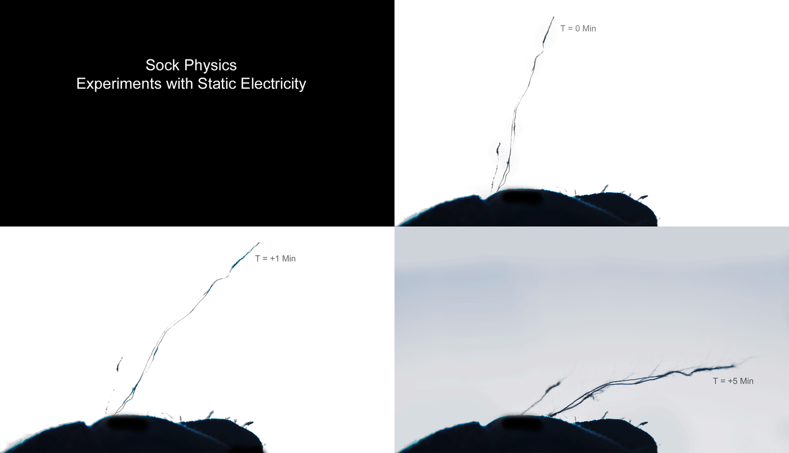
When I tossed my clothes into a pile for sorting, I  watched as a loose strand from one sock reached upward as to defy gravity but stayed tethered to the sock.   Even knowing why this is so (or at least one explanation) it fascinates.  Over the next few minutes I held off sorting the clothes and took a few photographs.

Fig 1: Back lit sock with strand balanced against gravity by the repulsive force of static electricity

Even more amazing (to me), was the fine structure in the hair-like appendages that stood in repulsion to the main strand due to the repulsive forces of like charges.  When electrons are removed from neutrally charged atoms, a net positive charge remains.  The force between like charges is a repulsive one so the individual strands are forced apart.

Fig 2: fine structure detail from Fig 1 showing small fibers of the sock in mutual repulsion.

A few minutes later, the long strand was clearly losing the battle against gravity as the collected charges slowly dissipated as nitrogen and oxygen molecules took them away.   

Fig 3: Strand 5 minutes later

Eventually, the rebellious strand lost its charge and rejoined the sock.  

Fig 4:  Composite showing positions of strand over 5 minutes as it loses charge and settles under the force of gravity

Fig 5: Mouse-click for animation 

All Aboard II

All Aboard II, a set on Flickr.

West Oakland's 16th Train Station was closed following Loma Prieta in 1989. The local train service has been relocated, but the 16th Street Train Station is gaining a new life as a center for community activities and special performances.

For more information, see http://www.indiegogo.com/16thStreetStation